Your browser doesn't support the features required by impress.js, so you are presented with a simplified version of this presentation.

For the best experience please use the latest Chrome, Safari or Firefox browser.

Convolutional Neural Network

Hao Su

Fall, 2021

Many slides are from Stanford CS231n

Agenda

    click to jump to the section.

    Limitations of Linear Classifiers

    Recap: Linear Classifier

    \[ f_{W,b}(x)=\underbrace{W}_{10\times 3072}\quad \underbrace{x}_{3072\times 1}+\underbrace{b}_{10\times 1} \]

    Recap: Loss Functions

    Given a training dataset $\{(x_i,y_i)\}_{i=1}^n$.
    • $f(x;\theta)$ to denote the classifier (e.g., linear classifier) parameterized by $\theta$.
    • $f_i(x;\theta)$ to denote the score for the $i$-th class
    • Then the loss function is \[ L(\theta)=-\frac{1}{n}\sum_{i=1}^n \log \left(\frac{e^{f_{y_i}(x_i;\theta)}}{\sum_j e^{f_j(x_i;\theta)}}\right) \]

    Problem: Linear Classifiers are not very powerful

    Linear classifiers only work when data points are linearly separable.
    Examples of linearly separable versus linearly non-separable:
    linearly separable
    linearly non-separable

    Motivation of Feature Extraction

    Image Feature Extraction

    Neural Networks

    The Original Linear Classifier

    (Before) Linear score function: $f=Wx$, where $x\in\R{D}$, $W\in\R{C\times D}$
    In practice, we will usually add a bias term.

    2-Layer Network

    (Before) Linear score function: $f=Wx$, where $x\in\R{D}$, $W\in\R{C\times D}$
    (Now) 2-layer Neural Network: $f=W_2\max(0, W_1x)$, where $x\in\R{D}$, $W_1\in\R{H\times D}$, $W_2\in\R{C\times H}$
    In practice, we will usually add a bias term at each layer, as well.

    3-Layer Network

    (Before) Linear score function: $f=Wx$, where $x\in\R{D}$, $W\in\R{C\times D}$
    (Now) 2-layer Neural Network: $f=W_2\max(0, W_1x)$, where $x\in\R{D}$, $W_1\in\R{H\times D}$, $W_2\in\R{C\times H}$
    or 3-layer Neural Network: $f=W_3\max(0,W_2\max(0,W_1x))$
    In practice, we will usually add a bias term at each layer, as well.

    Hierarchical Computation

    2-layer Neural Network: $f=W_2\max(0, W_1x)$
    • All dimensions of $h$ are computed from all dimensions of $x$; and all dimensions of $s$ are computed from all dimensions of $h$.
    • $W_1$ and $W_2$ are also called fully-connected layers (FC layers), and the network is also called a multi-layer perceptron (MLP).

    Why is $\max$ Operator Important?

    (Before) Linear score function: $f=Wx$
    (Now) 2-layer Neural Network: $f=W_2\fcolorbox{blue}{white}{$\max(0,$} W_1x)$
    The function $\max(0,z)$ is called the activation function.
    Q: What if we try to build a neural network without activation function?
    \[ f=W_2W_1x \]
    A: Let $W_3=W_2W_1\in\R{C\times H}$, then $f=W_3x$. We ended up with a linear classifier again!
    $\max$ operator introduces non-linearity!

    Activation Functions

    ReLU is a good default choice for most problems

    Example Feed-Forward Computation
    of a Neural Network

    
                            [REPLACE BY A TORCH CODE SNIPPET]
    # forward-pass of a 3-layer neural network:
    f = lambda x: 1.0 / (1.0 + np.exp(-x)) # activation function (use sigmoid)
    x = np.random.randn(3, 1) # random input vector of three numbers (3x1)
    h1 = f(np.dot(W1, x) + b1) # calculate first hidden layer activations (4x1)
    h2 = f(np.dot(W2, h1) + b2) # calculate second hidden layer activations (4x1)
    out = np.dot(W3, h2) + b3 # output neuron (1x1)
                            

    Learning a Neural Network: Log-Likelihood Loss (Recall)

    Given a training dataset $\{(x_i,y_i)\}_{i=1}^n$.
    • $f(x;\theta)$ to denote the classifier (e.g., linear classifier) parameterized by $\theta$.
    • $f_i(x;\theta)$ to denote the score for the $i$-th class
    • Then the loss function is \[ L(\theta)=-\frac{1}{n}\sum_{i=1}^n \log \left(\frac{e^{f_{y_i}(x_i;\theta)}}{\sum_j e^{f_j(x_i;\theta)}}\right) \]
    $\theta$: Weights $W_i$ and $b_i$ in all neural network layers

    Learning a Neural Network: Optimization (Recall)

    \[ L(\theta)=-\frac{1}{n}\sum_{i=1}^n \log \left(\frac{e^{f_{y_i}(x_i;\theta)}}{\sum_j e^{f_j(x_i;\theta)}}\right) \] Stochastic Gradient Descent (SGD)
    • A very simple modification to GD
    • At every step, randomly sample a minibatch of data points (e.g., 256 data points)
    • Compute the average gradient on the minibatch to update $\theta$

    Back-Propagation

    • So we need to compute the gradient of the neural network.
    • For example, in a 2-layer neural network \[ f_{W_1, W_2}(x)=W_2\max(0,W_1x), \] we need to compute the partial gradients with respect to each weight in $W_i$'s.
    • Gradient computation uses the chain rule of differentiation: \[ g(h(\theta_i))=\frac{\partial g}{\partial h}\frac{\partial h}{\partial \theta_i} \]
    • In network training, gradient computation by chain rule is called error back-propagation.

    Back-Propagation: Example Code

    [ADD PYTORCH CODES HERE]

    Full Implementation of Training a Neural Network

    [REPLACE BY TORCH CODE]

    Universal Approximation

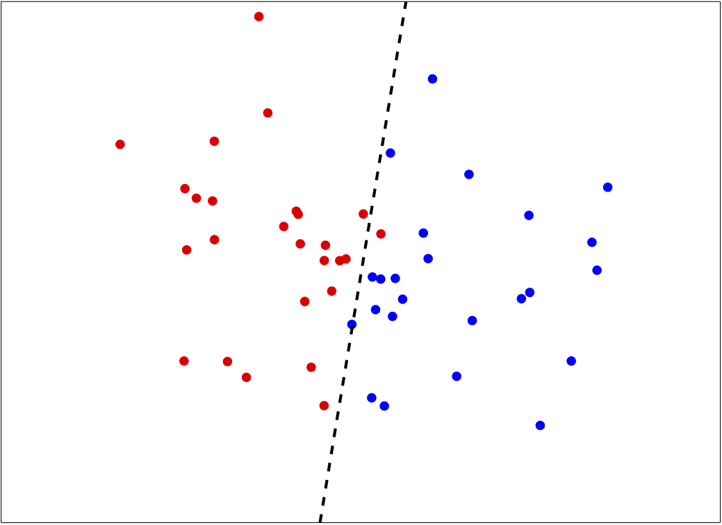
    Decision Boundaries of Linear Classifiers

    • Let us first restrict the discussions to binary classification
    • Recall that, the decision boundary of a linear classifier can only be straight lines.

    Decision Boundaries of Neural Networks

    Consider the 2-layer neural network: \[ f_{W_1, W_2}(x)=W_2\max(0,W_1x), \]

    Decision Boundaries of Neural Networks

    • We are able to create a very complex decision boundary by even a 2-layer neural network
    • In the following example, all the training data will have correct label predictions with 20 hidden neurons

    In fact, for any given dataset with non-conflicting labels, we can always add enough hidden neurons so that all the training data can be predicted correctly (but may fail on test data).

    Bias and Variance

    End