Recognition: Draw Understanding From Images

We take image classification as the example understanding task.
Example Image Classification Challenge (CIFAR10)
- Task: Given an image, label it as one of the predefined semantic categories
- In CIFAR10, each image is given as a $32\times 32\times 3$ matrix.

Recognition is Difficult
- Semantic gap: The gap between low-level machine readable data and high-level human readable representation
- Can we hard-code rules to do recognition by
if-else
? Usually very hard. - Let us try to describe the appearance of
cats

Challenge: Change of Viewpoint

Challenge: Illumination

Challenge: Deformation

Challenge: Occlusion

Challenge: Background Clutter

Challenge: Intraclass Variation

Train-Test Split
You might have heard that
I trained a machine learning model. What is training?
In machine learning for image classification, we have two sets of data: training data and testing data.
Example: In CIFAR10,
- training set: 50,000 images in total (5,000 images per category)
- test set: 10,000 images in total (1,000 images per category)
Machine Learning: Data-Driven Approach
- Collect a dataset of images and labels
- Use Machine Learning algorithms to train a classifier
- Evaluate the classifier on new images
def train(images, labels):
    # machine learning!
    return model
def predict(model, test_images):
    # use model to predict labels
    return test_labels
Stanford CS231n, Lecture 2
First classifier: Nearest Neighbor Method
 Distance metric:

Distance Metric to Compare Images
\[
d_1(I_1, I_2)=\sum_i |I_1^i-I_2^i| \tag{$L_1$ distance}
\]


Nearest Neighbor classifier

Nearest Neighbor classifier
Memorize training data
Memorize training data
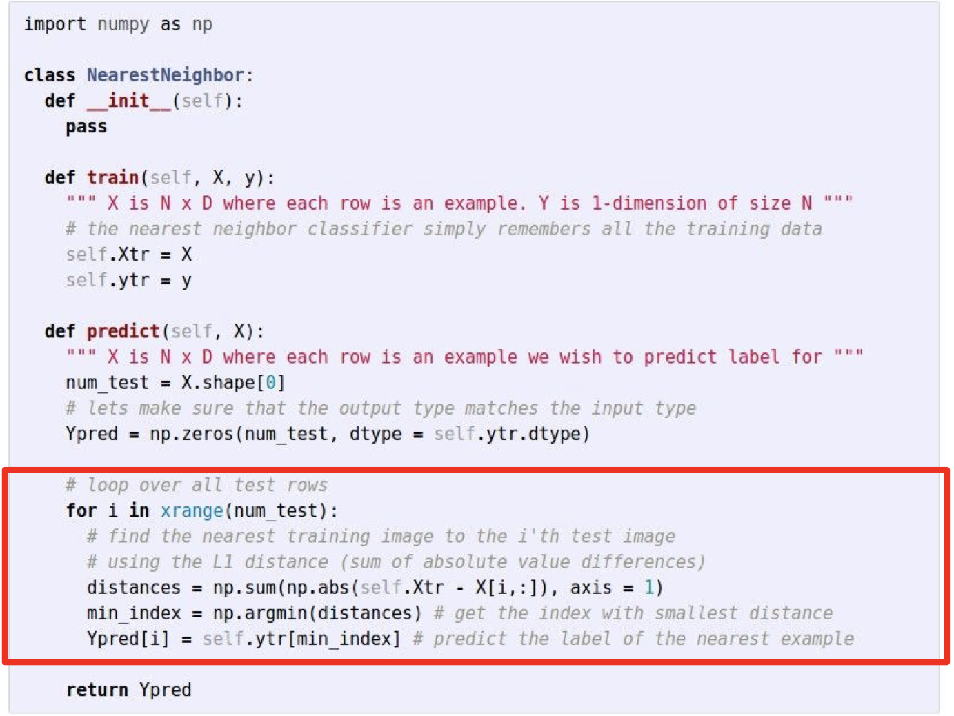
Nearest Neighbor classifier
For each test image:
Find closest train image
Predict label of nearest image
For each test image:
Find closest train image
Predict label of nearest image
Nearest Neighbor classifier
Q: With $N$ examples, how fast are training and prediction?
Q: With $N$ examples, how fast are training and prediction?
A: Train $\mathcal{O}(1)$, predict $\mathcal{O}(N)$.
This is bad: we want classifiers that are fast at prediction; slow for training is ok
Example Results on CIFAR10

Example Results on CIFAR10

Data Samples and Labels
- A data sample is a vector $x\in\R{n}$
- e.g., we can represent an image as a $32\times 32\times 3=3072$ dimensional vector
- The data sample $x$ belongs to one of $C$ predefined categories
- e.g., $C=3$ for boat/cat/plane
- We use an integer $y\in \{1,\ldots, C\}$ to represent the groundtruth label of $x$. Each number corresponds to a category.
- e.g., $y=1$ for boat, $y=2$ for cat, $y=3$ for plane

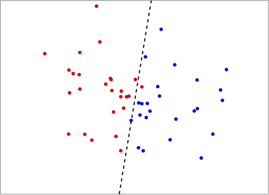
Geometric Visualization of a Classifier
- Consider a simplified classification problem: predict the label of 2D points on the plane.
- We plot the training data as points below. For each training data point $x$, the color indicates its class label.
- For any test point on the 2D plane, the predicted label by a nearest neighbor classifier is indicated by the color shading.

Linear Score Function
\[
f_{W,b}(x)=\underbrace{W}_{10\times 3072}\quad \underbrace{x}_{3072\times 1}+\underbrace{b}_{10\times 1}
\]

Example with an image with 4 pixels and 3 classes (cat/dog/ship):

Example with an image with 4 pixels and 3 classes (cat/dog/ship):

If $(W,b)$ is from a good classifier, it should give the highest score to the groundtruth class.
Geometric View of a Linear Classifier

Suppose: 3 training examples, 3 classes.
With some $(W,b)$ the scores $f_{W,b}(x)=Wx+b$ are:
With some $(W,b)$ the scores $f_{W,b}(x)=Wx+b$ are:
A loss function tells how good our current classifier is
Given a training set of examples
\[
\{(x_i, y_i)\}_{i=1}^{n_{train}}
\]
where $x_i$ is the image and $y_i$ is the label
Loss over the dataset is an average of loss over examples:
\[
L=\frac{1}{n_{train}}\sum_i L_i(f_{W,b}(x_i), y_i)
\]
Convert Scores into Probabilities by Softmax
Want to interpret raw classifier scores as probabilities
- Use the shorthand for the score vector: $s=f_{W,b}(x_i)$
- Turn $s$ into the predicted probability that a data belongs to class $k$ by the softmax function: \[ P(Y=k|X=x_i)=\frac{e^{s_k}}{\sum_j e^{s_j}} \]

cat
car
frog
car
frog
3.2
5.1
-1.7
5.1
-1.7
$\xrightarrow{\text{exp}}$
Probabilities must be >= 0
24.5164.0
0.18
$\xrightarrow{\text{normalize}}$
Probabilities must sum up to 1
0.130.87
0.00
Negative Log-Likelihood Loss
- We would like the probability of the groundtruth class to be maximized.
- Negative Log-Likelihood loss: Minimize $-\log P(Y=y_{groundtruth}|X=x_i)$ is equivalent to maximizing the predicted probability of the groundtruth class: \[ L_i=-\log\left(\frac{e^{s_{y_{groundtruth}}}}{\sum_j e^{s_j}}\right) \]
cat
car
frog
car
frog
3.2
5.1
-1.7
5.1
-1.7
$\xrightarrow{\text{exp}}$
Probabilities must be >= 0
24.5164.0
0.18
$\xrightarrow{\text{normalize}}$
Probabilities must sum up to 1
0.130.87
0.00
$\xrightarrow{-\log}$
Loss: $-\log P(Y=y_{groundtruth}|X=x_i)$
$L_i=-\log(0.13)=2.04$
Gradient Descent for Numerical Optimization
Consider the general optimization problem:
\[
\begin{aligned}
&\underset{x}{\text{minimize}}&& f(x)
\end{aligned}
\]

SGD with Momentum
\[
\theta^t = \beta \theta^{t-1} - (1-\beta) \alpha g
\]
$\alpha$: learning rate (e.g., $\alpha = 1e-4$)$\beta$: momentum (e.g., $\beta=0.9$)
$g$: gradient

Left — SGD without momentum, right— SGD with momentum.

Consider a 3-category classification problem (colored dots as training data).

Intepretation
- Colored lines: line equations of \[ \begin{align} 0&=w_1^Tx+b_1\\ 0&=w_2^Tx+b_2\\ 0&=w_3^Tx+b_3\\ \end{align} \]
- Vectors (normals of lines): $w_1$, $w_2$, and $w_3$
- $w_i$'s point to the direction that $f_i$'s give higher scores
Intepretation
- Colored regions: Where $f_i$ is higher than the scores of other categories
- Note that, the decision boundary between two categories are straight lines
Decision Boundary for Binary Classification
- Binary classification: When there are only two categories
- Decision boundary: A simple straight line
Hard Cases for a Linear Classifier
