Your browser doesn't support the features required by impress.js, so you are presented with a simplified version of this presentation.

For the best experience please use the latest Chrome, Safari or Firefox browser.

Optical Flow

Hao Su

Fall, 2021

Agenda

    click to jump to the section.

    Basic Idea of Structure from Motion

    Structure from Motion

    Pipeline of Multi-View 3D Reconstruction:
    1. Take photos from many views
    2. Identify points of interest from images
    3. Search for corresponding points in other images — this step becomes easier in a video
    4. Compute camera positions
    5. Estimate 3D point positions

    Structure from Motion

    Basic Idea

    • In a video, a point will move to a neighborhood in the next frame
    • Therefore, estimating correspondence in a video should be a relatively easy search task
    • However, we will show that, we can even locate the point without search or comparison!

    Representation of Video

    Video

    • A video is a subsequence of frames captured over time
    • Can be represented as a function $f(x,y,t)$, where $(x,y)$ indexes coordinates on the image plane, and $t$ indexes the time frame.

    Video

    • A real video sequence:

    Motion and Optical Flow

    General Idea of Flow Field

    Motion Field and Optical Flow Field

    • Assume that we use a video recorder to capture a moving star at $30$ frames per second
    • The star moves from $P_t\in\R{3}$ at frame $t$ to $P_{t+1}\in\R{3}$ at frame $t+1$
    • The corresponding pixel moves from $x_t\in\R{2}$ at frame $t$ to $x_{t+1}\in\R{2}$ at frame $t+1$

    Example of Optical Flow

    How Motion Field Causes Optical Flow

    The relative motion between objects and the camera can cause motion field
    • Object can move (e.g., cars are moving)
    • The movement of the camera also causes optical flow

    Optical Flow Caused by Camera Motion

    Optical Flow Caused by Camera Motion

    Not All Motion Causes Optical Flow

    Look at the following example:
    • The sphere has uniform surface material. When the sphere revolves, no motion is perceived.
    • Even if the object does not revolve, a moving light source can produce shading changes (fake motion)

    Estimation of Optical Flow

    Task Definition

    Question:
    • Given two subsequent frames, can we estimate the optical flow field $(u(x,y), v(x,y))$ between them?
    • $u(x,y):$ the $x$-offset of the flow vector
    • $v(x,y):$ the $y$-offset of the flow vector

    Key Assumptions of Optical Flow Estimation

    • Appearance constancy: Projection of the same point looks the same in every frame
    • Small motion: Points do not move very far
    • Spatial coherence: Points move like their neigbhors

    Key Assumptions: Appearance Constancy

    As the object moves, image measurements (e.g., brightness or color) in a small region remain the same: \[ I(x+u, y+v, t+1) = I(x,y,t) \]

    Key Assumptions: Small Motion

    The motion of the image patch is slow: \[ u\text{ and } v\text{ is small for }I(x+u, y+v, t+1) = I(x,y,t) \]

    Key Assumptions: Spatial Coherence

    In a neighborhood, the color/brightness of pixels are similar (because neighboring points are from the same object area, it is likely that the assumption is true): \[ I(x,y,t) \text{ is a smooth function at most locations} \]

    Summary of Key Assumptions

    • Brightness constancy: $I(x+u, y+v, t+1) = I(x,y,t)$
    • Small motion: $u\text{ and } v\text{ is small for }I(x+u, y+v, t+1) = I(x,y,t)$
    • Spatial coherence: $I(x,y,t) \text{ is a smooth function at most locations}$
    Recall the idea to characterizes that a function $f(x)$ is smooth (in fact, the definition of continuous):
    • When $x$ changes a bit, $f(x)$ only changes a bit
    We see that $I(x,y,t)$ is a function that is quite smooth!

    Optical Flow Constraints (grayscale images)

    By the smoothness of $I(x,y,t)$, we can take the first-order Taylor's expansion at $(x,y,t)$: \[ I(x+u,y+v,t+1)\approx I(x,y,t)+\frac{\partial I}{\partial x} u+\frac{\partial I}{\partial y} v+\frac{\partial I}{\partial t} \]
    Due to brightness constancy constraint, $I(x+u, y+v, t+1) = I(x,y,t)$. Therefore, \[ \frac{\partial I}{\partial x}u+\frac{\partial I}{\partial y}v+\frac{\partial I}{\partial t}=0\tag{brightness constancy constraint} \]

    Brightness Constancy Constraint

    \[ \frac{\partial I}{\partial x}u+\frac{\partial I}{\partial y}v+\frac{\partial I}{\partial t}=0 \]
    Connects the gradient of image w.r.t. space and w.r.t. time!

    Brightness Constancy Constraint

    \[ \frac{\partial I}{\partial x}u+\frac{\partial I}{\partial y}v+\frac{\partial I}{\partial t}=0 \]
    • Given a pixel $(x,y,t)$ in a video, $\frac{\partial I}{\partial x}(x,y,t)$, $\frac{\partial I}{\partial y}(x,y,t)$, and $\frac{\partial I}{\partial t}(x,y,t)$ are three known numbers.
    • Thus it is a linear equation over $u$ and $v$.
    • Obviously, $(u, v)$ cannot be uniquely determined by this single equation!
    \[ \frac{\partial I}{\partial x}u+\frac{\partial I}{\partial y}v+\frac{\partial I}{\partial t}=0 \] What is $(\frac{\partial I}{\partial x}, \frac{\partial I}{\partial y})$? Gradient, the direction that function value increases fastest! Orthogonal to edge direction.
    Suppose that $(u_0,v_0)$ satisfies the brightness constancy constraints at $(x, y, t)$. What are other solutions?
    For any $(\Delta u, \Delta v)$ such that $\frac{\partial I}{\partial x}\Delta u + \frac{\partial I}{\partial y}\Delta v=0$, $(u+\Delta u, v+\Delta v)$ must also be a solution!
    In other words, $[\frac{\partial I}{\partial u}, \frac{\partial I}{\partial v}]^T \perp [\Delta u, \Delta v]^T$.
    But $[\frac{\partial I}{\partial u}, \frac{\partial I}{\partial v}]^T$ is orthogonal to edge direction. So $[\Delta u, \Delta v]^T$ is along the edge direction!
    \[ \frac{\partial I}{\partial x}u+\frac{\partial I}{\partial y}v+\frac{\partial I}{\partial t}=0 \] Suppose that $(u_0,v_0)$ satisfies the brightness constancy constraints at $(x, y, t)$.
    • For any $(\Delta u, \Delta v)$ such that $\frac{\partial I}{\partial x}\Delta u + \frac{\partial I}{\partial y}\Delta v=0$, $(u+\Delta u, v+\Delta v)$ must also be a solution!
    • $[\Delta u, \Delta v]^T$ is along the edge direction!
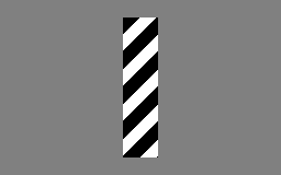
    The feeling is pixels are moving downwards
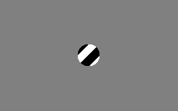
    The feeling is pixels are moving towards bottom-right

    Addressing Ambiguity in Brightness Constancy Constraint

    Spatial Coherence

    First-order expansion of $I(x,y,t)$ provides one equation for two variables $(u,v)$ at a pixel at $(x,y,t)$. How can we get more equations for the pixel?
    • We add an additional assumption: Neighboring pixels have the same $(u,v)$.

    Spatial Coherence

    • If we take a $5\times 5$ neighborhood window around the pixel, at each pixel in the window we have an equation for $(u,v)$. So we have 25 equations in total.
    • Denote $I_x(p)= \frac{\partial I}{\partial x}(p)$, $I_y(p)= \frac{\partial I}{\partial y}(p)$, $I_t(p)= \frac{\partial I}{\partial t}(p)$ where $p=(x,y,t)$. \[ \frac{\partial I}{\partial x}u+\frac{\partial I}{\partial y}v+\frac{\partial I}{\partial t}=0\Rightarrow [I_x(p), I_y(p)] \begin{bmatrix} u\\v \end{bmatrix}+I_t(p)=0 \]
    • Constraints in matrix form \[ \begin{bmatrix} I_x(p_1) & I_y(p_1)\\ I_x(p_2) & I_y(p_2)\\ \vdots & \vdots\\ I_x(p_{25}) & I_y(p_{25}) \end{bmatrix} \begin{bmatrix} u \\ v \end{bmatrix}= - \begin{bmatrix} I_t(p_1)\\ I_t(p_2)\\ \vdots\\ I_t(p_{25}) \end{bmatrix} \]

    Spatial Coherence

    \[ \underbrace{ \begin{bmatrix} I_x(p_1) & I_y(p_1)\\ I_x(p_2) & I_y(p_2)\\ \vdots & \vdots\\ I_x(p_{25}) & I_y(p_{25}) \end{bmatrix}}_{A} \underbrace{ \begin{bmatrix} u \\ v \end{bmatrix}}_{d}= \underbrace{ - \begin{bmatrix} I_t(p_1)\\ I_t(p_2)\\ \vdots\\ I_t(p_{25}) \end{bmatrix}}_{b} \] Written compactly: \[ Ad=b \] Overdetermined system. Can be solved by least square: \[ d = (A^TA)^{-1}A^Tb \]
    \[ d = (A^TA)^{-1}A^Tb \] \[ A = \begin{bmatrix} I_x(p_1) & I_y(p_1)\\ I_x(p_2) & I_y(p_2)\\ \vdots & \vdots\\ I_x(p_{25}) & I_y(p_{25}) \end{bmatrix},\quad b=- \begin{bmatrix} I_t(p_1)\\ I_t(p_2)\\ \vdots\\ I_t(p_{25}) \end{bmatrix} \] \[ A^TA= \begin{bmatrix} I_x(p_1) & I_x(p_2) & \cdots & I_x(p_{25})\\ I_y(p_1) & I_y(p_2) & \cdots & I_y(p_{25})\\ \end{bmatrix} \begin{bmatrix} I_x(p_1) & I_y(p_1)\\ I_x(p_2) & I_y(p_2)\\ \vdots & \vdots\\ I_x(p_{25}) & I_y(p_{25}) \end{bmatrix}= \begin{bmatrix} \sum_i I_x(p_i)I_x(p_i) & \sum_i I_x(p_i)I_y(p_i)\\ \sum_i I_x(p_i)I_y(p_i) & \sum_i I_y(p_i)I_y(p_i) \end{bmatrix} \] \[ A^Tb = \begin{bmatrix} I_x(p_1) & I_x(p_2) & \cdots & I_x(p_{25})\\ I_y(p_1) & I_y(p_2) & \cdots & I_y(p_{25})\\ \end{bmatrix} \left(- \begin{bmatrix} I_t(p_1)\\ I_t(p_2)\\ \vdots\\ I_t(p_{25}) \end{bmatrix}\right)= \begin{bmatrix} -\sum_i I_x(p_i) I_t(p_i)\\ -\sum_i I_y(p_i) I_t(p_i) \end{bmatrix} \]

    Solutions for Estimating Optical Flow

    To sum up, given $(x,y,t)$ and its neighborhood, we can estimate the flow vector $ d= \begin{bmatrix} u\\v \end{bmatrix} $ that points from $(x,y,t)$ to $(x+u,y+v,t+1)$ by: \[ d = (A^TA)^{-1}A^Tb \] where \[ A^TA= \begin{bmatrix} \sum I_xI_x & \sum I_xI_y\\ \sum I_xI_y & \sum I_yI_y \end{bmatrix}, \quad A^Tb = - \begin{bmatrix} \sum I_x I_t\\ \sum I_y I_t \end{bmatrix} \]

    Stability Analysis

    Q: Which pixels will give us better estimations?

    Statistical View of Image Formation

    In computer vision, we often take a statistical view to treat images. We often assume that the observation is corrupted by some unknown noises.
    For example,
    • dirts on the lens
    • imperfection of optics sensor and signal processing in the camera
    • blur caused by object motion
    • caustics caused by material refraction and reflection

    Statistical View of Image Formation

    For example, additive noise model assumes that \[ I(x,y,t)=I^{gt}(x,y,t)+\epsilon \] where $I^{gt}(x,y,t)$ is the hypothesized groundtruth pixel value, and $\epsilon$ is a random noise sampled from a distribution $\mathcal{P}$.

    Statistical View of Image Formation

    Recall that \[ A^TA= \begin{bmatrix} \sum I_xI_x & \sum I_xI_y\\ \sum I_xI_y & \sum I_yI_y \end{bmatrix} \] Since every pixel value is a random variable, $A^TA$ is in fact a random matrix (a matrix that all elements are random variables).

    Conditions for Solvability

    • To estimate the flow vector $d = (A^TA)^{-1}A^Tb$, the key challenge is to compute $(A^TA)^{-1}$
    • First of all, $A^TA$ is a symmetric matrix

    Spectral Decomposition Theorem

    For any symmetric matrix $M\in\R{n\times n}$, we have a theorem from linear algebra that, \begin{equation} M=V\Lambda V^T \tag{spectral decomposition theorem} \end{equation} where
    • $\Lambda\in\R{n\times n}$: a diagonal matrix whose diagonal entries are eigenvalues
    • $V\in\R{n\times n}$: an orthonormal matrix such that the $i$-th column is the eigenvector corresponding to the $i$-th eigenvalue

    Conditions for Solvability

    • Assume that $A^TA=V\Lambda V^T$, then $(A^TA)^{-1}=V\Lambda^{-1}V^T$
    • If $V=[v_1, v_2]$ where $v_1, v_2\in\R{2\times 1}$, then \[ (A^TA)^{-1}=[v_1\ v_2] \begin{bmatrix} \frac{1}{\lambda_1} & 0 \\ 0 & \frac{1}{\lambda_2} \\ \end{bmatrix} \begin{bmatrix} v_1^T\\v_2^T \end{bmatrix}= \frac{1}{\lambda_1}v_1v_1^T+\frac{1}{\lambda_2}v_2v_2^T \]
    • As we analyzed before, there is randomness in $A^TA$. In fact, there are also randomness in $\lambda_1$ and $\lambda_2$. They are random numbers near the groundtruth value.
    • Let us assume that $\lambda_1>\lambda_2>0$.
      • If $\lambda_1$ and $\lambda_2$ are both big. Good!
      • If $\lambda_2\approx 0$, then $\frac{1}{\lambda_2}$ will be very unstable due to randomness and numerical errors. Thus $(A^TA)^{-1}$ will be very unstable!

    Conditions for Solvability

    Based on the analysis, flow estimation is the most reliable
    when the eigenvalues $\lambda_1$ and $\lambda_2$ of \( A^TA= \begin{bmatrix} \sum I_xI_x & \sum I_xI_y\\ \sum I_xI_y & \sum I_yI_y \end{bmatrix} \) are both large.
    Q: What is the intuition of this result?

    Review: Diagram of Cornerness

    Let $M=\sum \begin{bmatrix} I_x I_x & I_x I_y\\ I_x I_y & I_yI_y \end{bmatrix}$, suppose the eigenvalues of $M$ are $\lambda_1$ and $\lambda_2$.
    Good points to track are Harris corner points!

    Low Textured Area

    Edge

    Corner

    Example for Lukas-Kanade Face Tracking

    End